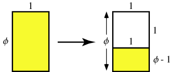
The Fibonacci numbers are generated by setting \(F(0)=0, F(1)=1\), and then using the recursive formula \[ \begin{equation} F(n) = F(n-1) + F(n-2) \end{equation} \] to get the rest. Thus the sequence begins: \(0, 1, 1, 2, 3, 5, 8, 13, 21, 34,\) ...
Leonardo of Pisa, known as Fibonacci, introduced the Fibonacci sequence to European mathematics in his 1202 book Liber Abaci. It is thought to have arisen even earlier in Indian mathematics.
Appearance in Nature
I have read many claims of fibonacci numbers appearing as spirals in galaxies and in plant life as phyllotaxis of leaves, because spiral structures allow organisms to grow without changing shape and optimizes the consumption of water and sun light. Also the pyramids, ancient greek architecture is said to utilize the golden ratio. The golden ratio was used widely in the Renaissance in paintings. I will describe the math with some programming in the following.
You can look all these mystical subjects up yourself, if you wish to study this further.  the image is from John Wilsons page at University of Georgia.
How du you calculate the numbers?
Because of all these claims which I have read, I thought it would be interesting to know a bit more about the mathematical nature of the called golden ratio and the fibonacci numbers and spiral. Therefore, it would be an interesting way for me to learn some more coding in Python. There are mainly the recursive way of calculating the sequence and then two non recursive ways of calcuating for example fibonacci number one hundred.
For example to calculate the first \(25\) numbers.
# A recursive method
n=25;
def fib(n):
    if n < 2:
        return n
    else:
        return fib(n-1) + fib(n-2)
print [fib(i) for i in range(n + 1)]
The golden ratio
However, if I wanted the 100th term of this sequence and had no computer, it would take lots of intermediate calculations with the recursive formula to get a result.
There is an exact formula for the n\(th\) term. This formula is attributed to Binet in 1843: \[
\begin{equation}
F(n) = \frac{\Phi^n - (-\Phi)^{-n}}{\sqrt{5}}
\end{equation}
\] \(\Phi=\frac{1+\sqrt{5}}{2}\approx1.618\) is called the golden ratio. 
The higher up in the sequence, the closer two consecutive Fibonacci numbers of the sequence divided by each other will approach the golden ratio. That is \(\frac{F(n)}{F(n-1)}\approx\Phi\)
# Using Binet's formula
n=25
def fib2(n):
    phi = (1 + 5**0.5)/2.; print "phi = ", phi
    return (((phi**n - (1-phi)**n) / 5**0.5))
print "f(n) = %1.0f" %fib2(n)
This can in fact also be implemented with matrix algebra in the following form: \[ \left[ \begin{array}{l} F( n )\\F(n-1) \end{array} \right] = Ax = \begin{equation} \begin{bmatrix} 1 & 1 \\ 1 & 0 \\ \end{bmatrix} \left[ \begin{array}{l} F(n-1)\\F(n-2) \end{array} \right]\\ \end{equation} \] or simply just this form will contain the desired number. \[ \begin{equation} A^n = \begin{bmatrix} 1 & 1 \\ 1 & 0 \\ \end{bmatrix}^n \end{equation} \] A actaully has the eigenvalues \(\lambda=\frac{1\pm\sqrt{5}}{2}\). More info on this here. Finally, I will demonstrate a python program which plots the fibonacci spiral.
Programming a plot of Fibonacci spiral in Python
A Fibonacci spiral approximates the golden spiral using quarter-circle arcs inscribed in squares with sides with size of Fibonacci-numbers. I have made an approximation of the golden spiral created by drawing circular arcs connecting the opposite corners of squares in the Fibonacci tiling; this one uses squares of sizes 1, 1, 2, 3, 5, 8, 13, 21, 34 and 55 as plotted in the labels.
"""
Fibonacci squares and spirals by the use of artist, by Jacob Møller
http://matplotlib.org/examples/shapes_and_collections/artist_reference.html
"""
import matplotlib.pyplot as plt; plt.rcdefaults()
import numpy as np
import matplotlib.pyplot as plt
import matplotlib.path as mpath
import matplotlib.lines as mlines
import matplotlib.patches as mpatches
from matplotlib.collections import PatchCollection

def fib(n):
    if n < 2:
        return n
    else:
        return fib(n-1) + fib(n-2)

def label(xy, text, j):
    y = xy[1] - 0.025 # shift y-value to center label
    plt.text(xy[0], y, text, ha="center", family='sans-serif', size=j)

fig, ax = plt.subplots(); patches = []

xy = np.array([0, 0]); c = xy; i=1; t = numpy.array([270, 0])
for j in range(1,7+4):
    t += 90;
    if i == 5: i=1;
    if i==1:
        xy = xy + [ -fib(j-2)    , fib(j-1) ];     c = c + [ -fib(j-2), 0         ];
    if i==2:
        xy = xy + [ -fib(j)      , -fib(j-2)];     c = c + [0         , -fib(j-2) ];
    elif i==3:
        xy = xy + [ 0            , -fib(j)  ];     c = c + [ fib(j-2) , 0         ];
    elif i==4:
        xy = xy + [ fib(j-1)     , 0        ];     c = c + [ 0        , fib(j-2)  ];

    # Add a wedge
    rect = mpatches.Wedge([c[0],c[1]], fib(j), t[0] , t[1]   , ec="none")
    patches.append(rect)

    # Add a rectangle
    rect = mpatches.Rectangle([xy[0],xy[1]], fib(j), fib(j), ec="none"); patches.append(rect); i+=1;
    label( xy+[0.5*fib(j),  0.5*fib(j)], "%s"%fib(j), j*2)

colors = np.linspace(0, 0, 0)
collection = PatchCollection(patches, cmap=plt.cm.hsv, alpha=0.9); collection.set_array(np.array(colors)); ax.add_collection(collection)
plt.axis('equal'); plt.axis('off'); plt.grid('off');plt.show();
Yes, That was it. Feel free to use the code for your amusement!
...
